


Magnetic Resonance Imaging is the best method for non-invasive imaging of soft tissue anatomy, saving countless lives each year. It is regarded as the gold standard for diagnosis of mild to moderate traumatic brain injuries. However, conventional MRI relies on very high, fixed strength magnetic fields (> 1.5 T) with parts-per-million homogeneity, which requires very large and expensive magnets. The overwhelming technological trend in MRI has been toward ever higher magnetic fields [1] because the signal (sample magnetization) and sensitivity of the Faraday detectors traditionally used scale with the applied magnetic field (readout frequency). [2] Thus, bigger fields have been widely accepted as the only way to obtain quality images, but they come with a price. High-field MRI is a method that can only be used in highly controlled settings in well-funded medical centers where such large magnetic fields can be generated and do not pose a hazard. [3,4] MRI machines weigh many tons, cost $3-5 million, and typically require 100-1,000 liters of cryogens annually. The high magnetic fields also restrict access in other ways. Traditional highfield MRI is not available in rural settings, is not deployable to emergency situations or battlefield hospitals and is more expensive than what poor and developing countries can afford—leaving billions of people without access to this powerful diagnostic tool. Subjects with unknown medical histories, such as unconscious soldiers with possible shrapnel injuries, cannot be imaged because of the potential hazards of heating or moving metal in the body, due to the radio-frequency fields and the strong magnetic gradients. Even non-ferrous metal significantly distorts a high-field MRI, precluding imaging of those with medical implants. In this article, progress toward developing a portable Battlefield MRI machine based on Superconducting Quantum Interference Device sensor technology and ultra-low-field MRI techniques developed at Los Alamos National Laboratory will be discussed. This device requires only 10s of liters of cryogens annually, makes use very simple, and has light field generation, 10-100 times less than a traditional MRI machine. Imaging of the human brain at fields 10,000 times lower than traditional MRI, using a pulsed-field method, will be demonstrated along with the capability for imaging injuries as small as a few millimeters, including brain bleeding and hydrocephalus, via the use of a validated model. Operation in the presence of metal, or even through metal, compatibility with other medical equipment and brain imaging modalities as well as the potential for systems that can be easily deployed (e.g. truck or helicopter) will be discussed.
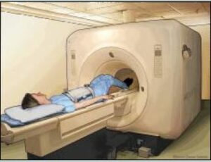
Illustration of MRI of the abdomen. (Image from the National Institutes of Health/Released)
Background:
Traumatic brain injuries are among the most devastating injuries on the battlefield, accounting for 15-25 percent of battlefield injuries since WWII. [5] The increasing incidence and effectiveness of improvised explosive devices in contemporary conflict suggests the problem is likely to get worse. [6] Since 2000, more than 300,000 U.S. military service members worldwide have sustained a TBI. Soldiers today have stronger armor and can survive close range explosions that would have killed soldiers in earlier wars. They also have access to rapid medical care for other injuries and many quickly return to combat. However, head injuries that do not involve obvious wounds or loss of consciousness, which is often the case for mild TBIs, or concussions, may go unnoticed. Although many patients completely recover from concussions, a fraction can have long-term effects, including mood disorders and depression. Some studies suggest TBIs can increase the risk of post-traumatic stress. [7]
Even when a head injury is suspected, there are few options for detection in a combat setting. Computerized tomography scanners, which use x-rays, are available in many combat support hospitals, but are not efficient at detecting the swelling or microscopic bleeding that may be associated with concussions. MRI is often better at identifying these microscopic changes. [8] However, the closest MRI to currently deployed service members in the Middle East and Afghanistan is at the U.S. military medical center in Landstuhl, Germany. An experiment in using traditional MRI in Afghanistan showed the machines were effective, but had to be pulled because of the high cost of maintaining conventional MRI in theater. [9]
Traditional MRI machines have multiple advantages for detecting changes in soft tissue, and it has been shown early intervention for even mild brain injuries can significantly improve a patient’s longterm prognosis. However, these machines are expensive, and the high magnetic fields are not safe for injuries involving metal (e.g., shrapnel), which rules out unconscious patients with an unknown medical history. Can weaker magnetic fields be used to image changes in soft tissue?
In the early years of MRI, lower field systems were used. MRIs had fields in the range of 10 to 100 mT and were largely based on permanent magnets, but these systems were expensive to maintain and very heavy. As superconducting magnet technology became available, systems stayed heavy and expensive, but the magnetic field strength, and thus image quality, went higher. What happens if the fields are even lower than mT? At much lower magnetic field strengths, it seemed that the signal was so poor true imaging would be impossible. That is until about 10 years ago when convergence or breakthroughs in sensor technology and magnetic field cycling methods made imaging at very low readout (i.e., earth’s magnetic field), ultra-low field MRI possible and practical.
In the early 2000s, John Clarke’s group at University of California, Berkeley showed MRI at ultra-low magnetic fields of ~100 mT and Larmor frequencies of kHz was possible by combining detection based on the superconducting quantum interference device, SQUID, with pre-polarization methods. [2] The SQUID is arguably the world’s most sensitive detector of magnetic fields. [10] Prepolarization (or field cycling) relies on using a higher magnetic field for a brief (a few seconds or less) amount of time to recruit signal. The actual MRI imaging, however, is done at a much lower magnetic field [11] that is easier to support, safer and much less homogeneous. [12] Since that time, Los Alamos National Laboratory and others have performed several compelling demonstrations of ULF MRI, especially for anatomical imaging of the brain. [13-16] Although the trend in MRI justifiably continues to be towards higher and higher magnetic fields, with 3 T now routine, to benefit from signal that scales as the magnetic field is squared, B2, the promise of unique applications enabled by the benefits of the ULF regime remains. These include narrow line widths, unique tissue contrast, reduced susceptibility artifacts, compatibility with magnetoencephalography (MEG, a sensitive technique for measuring brain activity by the magnetic fields produced from active neurons) and imaging in the presence of metal to name a few. It remains to be seen, one might speculate these benefits combined with the relaxed requirements for magnetic field generation will enable ULF MRI systems to be utilized clinically or perhaps in situations where traditional MRI cannot go. Examples include emergency response where the exclusion of metal is not possible or places where the cost and infrastructure of high-field MRI systems cannot be borne. To be able to achieve a diagnostic quality MRI at ultra-low fields would be truly revolutionary with regard to where MRI could go and who could have access.
However, to make such speculations reality, a few key facts must be overcome. Although much of the required core technology has been demonstrated, ULF MRI systems still suffer from long imaging times and relatively poor quality images, and they have been confined to the research and development laboratory because of the strict requirements for a low noise environment isolated from almost all ambient electromagnetic fields. The goal of the work presented here was to develop a ULF MRI system functional prototype that will exploit the inherent advantages of the approach with an eye toward enabling increased accessibility. The results from a seven-channel, SQUID-based system that achieves a prepolarization field of 100 mT over a 20 x 20 x 20 cm3 volume, powers all magnetic field generation from standard MRI amplifier technology, and uses off-the-shelf data acquisition are presented. As the ultimate goal is unshielded operation, a seven-channel system that performs ULF MRI outside of a heavy magnetically-shielded enclosure will also be demonstrated. In this paper, preliminary images and characterization of the performance in the context of a model are presented.
How MRI works
The fundamental principle behind MRI is to magnetize (polarize) a sample with non-zero nuclear spin in a large magnetic field. In our case, as in the majority of MRI machines, the nucleus in question is the proton found in the water, which is abundant in human tissue. Simply, one can think of the protons (or hydrogen nuclei in water) as being tiny bar magnets. When an external magnetic field is applied, a small number of the protons line up with the field, producing a magnetization. This magnetization can then be manipulated by subsequent application of magnetic fields to produce a measurable signal at a unique (Larmor) frequency w0, which is specific to the measurement (readout) magnetic field B0 and the type of nuclei,
![]() , (1)
, (1)
where g is the gyromagnetic ratio of the nuclei. In nearly all anatomical MRI, the sample is typically the spin ½ protons (hydrogen) found in water inside the body, thus g = 42.6 MHz/T. In our subsequent discussion, we will largely rely on the more general term “spin,” but for all the anatomical imaging described below, we mean the proton signal from water in the subject under study.
In traditional high field MRI typically found in hospitals, the subject is placed inside a large, highly uniform (parts per million), fixed strength, usually a superconducting, magnet of 1.5 or 3 T. Once in the field, the spins align to produce a net magnetization over a period of time, T1, which is very sensitive to the local chemical environment of the spins. After aligning, the spins can be “tipped” by an appropriately applied magnetic field pulse at the Larmor frequency. Once tipped, the spins rotate at the Larmor frequency, producing a time varying magnetic field that can be measured. The magnetization decays as the spins de-phase (relax) or get out of alignment due to local variations in the magnetic field. This relaxation time is known as T2. It is sensitive to both the uniformity of the applied fields and the chemical environment. Nearly all MRIs derive their information from a combination of spin density (how much hydrogen) and differences in T1 and T2 between tissues. It is T1 and T2 that make MRI so effective at distinguishing between tissue types.
In traditional MRI, the polarization, Bp, and measurement, Bm, magnetic field are the same and referred to as B0. A typical high field MRI would have a proton Larmor frequency of ~ 64 – 128 MHz. Practically, the higher the polarizing magnetic field achieved the better the signal. This is because the sample equilibrium magnetization, Bp.
The increased signal can be used for faster acquisition and higher resolution images. An additional motivation for high magnetic fields is that the performance of Faraday coils used as detectors in high field MRI, increases with magnetic field strength. [17] Thus, trying to perform conventional MRI at lower magnetic field strengths, where coil noise dominates, results in a penalty in acquired signal that scales as ~![]() .
.
The principal aim of all MRI is to spatially encode the signal properties (e.g. T1, T2, or spin density) underlying the information available in the images. In general, the physical principles used for ULF MRI are similar to those for traditional MRI. The main differences are: less signal and longer measurement time; different requirements for generation and manipulation of magnetic fields (which enable novel pulse sequences, but introduce new demands); differences in detector technology (i.e. SQUID vs. Faraday coil); and differences in T1 contrast. Here, we briefly review some fundamental concepts in MRI that will be helpful in highlighting the differences between HF and ULF approaches. An excellent and far more complete description of conventional MRI is found in Ref. [18].
Because the Larmor frequency over the sample depends on the spatial profile of the applied magnetic field over the sample (see Equation (1)) to produce an image, a magnetic field gradient G(t) (assumed to be a linear gradient for these discussions) that causes the frequency to vary in a known way was intentionally applied, such that
![]() (2)
(2)
The fact that the frequency of the MRI signal varies in space and a judicious application of field gradients, known as a pulse sequence, are used to develop a trajectory through image space and acquire a spatially encoded representation of the magnetization. By appropriate choice of pulse sequence, certain tissues can be highlighted or suppressed based on their T1 or T2.
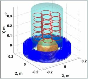

Figure 1. a) The sensor system (red) and cryostat (cyan), as well as the pre-polarization coil (blue) and location of the top of the head being imaged are shown. b) Schematic of the MRI coil set. Note the polarization field coil is not shown for simplicity. The figure is from Reference 24. (Released)
About ULF MRI
To make MRI work at ULF, requires addressing the loss of signal with magnetic field in two primary ways. First, there is a method of pulsed pre-polarization at higher fields (0.01 – 0.1 T) to increase the signal by increasing magnetization [19]. Unlike pulsed field applications with a tuned Faraday coil, in which signal scales as BmBp , [20] an un-tuned SQUID detects the signal that scales as Bp, while sensor noise is ~ 1 fT/`Hz from Hz – MHz. [17]
To help frame the discussion, in Figure 1 a schematic of the ULF MRI system [21] that was used for obtaining brain images is presented. A photograph of the system is shown in Figure 2. In the upper panel of Figure 1, a model depicting the layout of the cryostat, which holds the SQUID sensors (cooled with ~ 10 L of liquid helium), the pre-polarizaton coil, and the location of the human head being imaged, is shown. The sensor array [21] of seven SQUIDs connected to second-order axial gradiometers with pickup loop diameter and baseline ~90 mm are arranged as in the upper panel of Figure 1. An array of seven SQUIDs is used to improve the signal-to-noise and/or enable implementation of parallel imaging methods to speed the image acquisition [22].
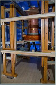
Figure 2. Photograph of the shielded system. (Courtesy of Michelle Epsy, LANL/Released)
The upper panel of Figure 1 and 2 also show the pre-polarization, or Bp coil, used to generate the sample magnetization. In the lower panel of Figure 1, the geometry of the remainder of magnetic field generation coils used to produce and spatially encode the MRI signal is presented. Bm denotes the measurement of the magnetic field coils along the z-axis. The additional Gx,y,z coils are for gradient encoding in the dBz/dx,y,z directions, respectively. As shown in Figure 2, the two coils wrapping around the outside of the system can also be seen (not shown in the lower panel of Figure 1 for simplicity). These are field cancellation coils designed to counteract any transient magnetic fields induced by pulsing the Bp coil. In HF MRI, there is a single fixed field providing both Bp and Bm, typically provided by a large superconducting magnet. In ULF MRI, the field generation is typically produced by simple electromagnets. This allows for different field orientations and strengths provided by separate Bp and Bm coils. Although it is not obvious from the photograph, the MRI system shown in figure 2 resides inside a large, magnetically shielded enclosure made of sandwiched layers of aluminum and a high permeability metal known as “mu-metal.” This provides a pristine magnetic field environment, but makes the system quite large and not mobile. Thus, removal of the requirement for shielding becomes quite important for mobility. However, it is important to first see what ULF MRI can do under “ideal” circumstances. A more complete discussion of this system is found in Ref. [21], and the issues and opportunities in ULF MRI can be found in Refs. [2] [23] or [24].
Results for shielded MRI
Almost everything about a ULF MRI system can be modeled, with the exception of the values of T1 and T2 at ULF, which can be complicated to predict and need to be measured. What then is the absolute best one can expect? Current state of the art research has shown that achieving pre-polarization fields of ~ 100 mT over the sample volume are challenging but reasonable. While, in principle, SQUIDs are capable of < 1 fT/`Hz noise, in practice it has been a struggle to see better than ~ 1.5 fT/`Hz in the presence of the energized field coils. That is taken to be the starting point. Using the parameters listed in Table I for the ULF MRI system shown in Figures 1 and 2, a model can be developed to determine the best image that could be obtained. The result is shown in Figure 3. The model is described more completely in Reference 21. The T1 and T2 contrast times used were experimentally measured previously [13,25]. The values from [13] were used in the model. The image quality is still rather poor. However, a sequence with a polarization time of 0.5 s, Fig. 3f, shows good contrast for a 1 cc inclusion with the relaxation properties of 50 percent blood and 50 percent brain tissue, indicating sensitivity to bleeding in the brain.

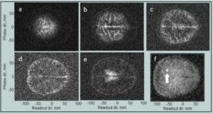
Fig. 3 a–e). Simulated ULF MRI of the brain with parameters from Table I. (f). Slice at 30–45 mm depth for pre-polarization of 0.5 s shows sensitivity to a one cm diameter inclusion (arrow) simulating bleeding. Data are from Reference 24. (Released)
In Figure 4, the experimental results for the same pulse sequence are presented. The long polarization time (4 s) means the images are primarily sensitive to cerebral spinal fluid. The total imaging time was 67 minutes compared to the ~10s of minutes typical for high field MRI. The length was due to long polarization and a 50% duty cycle to avoid overheating the Bp coil. This could be reduced to ~ 30 minutes once those issues are addressed. The spatial resolution for a slice was 2.1 × 2.4 mm2 with 15 mm slice thickness, whereas conventional MRI is able to achieve 1×1 mm2 with 5 mm slice thickness. The image signal-to-noise ratio for the second slice of simulated and measured data, calculated using the single-image measurement method [26], [Figure 3b and Figure 4b] was ~ 10 for both. Although different brains are used in the model [Figure 3] and the experimental data [Figure 4], the agreement between them is excellent, indicating the system is performing as expected.
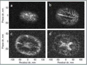
Figure 4. a–d) ULF MRI of the human brain, 15 mm thick transverse slices progressing in depth. The lower two slices are de-noised with a Golay filter. Data are from Reference 24. (Released)
Results for unshielded MRI
While the images shown in Figures 3 and 4 are able to distinguish major anatomical features and bleeding, the location of the system inside the 3x3x4 m3 magnetically shielded room will not enable this system to be portable or inexpensive.
To this end, a second system with no external metal shielding was designed. Instead this system is surrounded by three pairs of coils located in x-y-z that are used to cancel out the earth’s magnetic field and other unwanted ambient magnetic fields. A photograph of this system is shown in Figure 5. The ULF MRI working in an unshielded environment consisted of gradient and measurement field coils of the same kind as described in [27]. The cryostat and insert were the same 7-channel system as used in References 14 and 15. To test the performance of this system, a phantom brain was created using a mold [28] with the different compartments made from gelatin and agar designed to mimic the T2 times of brain tissue. Figure 6 shows a photograph of the phantom. The T2 was ~ 120 ms for the bulk and T2 ~ 300 ms for inclusions. Food coloring was used for visual enhancement. Not visible in Figure 6 are small ~ 1cc inclusions also at 300 ms, designed to simulate bleeding.
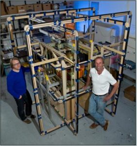
Figure 5. The Los Alamos Battlefield MRI Protype (Courtesy of LANL/Released)
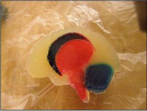
Figure 6. Photograph of the gelatin-agar brain phantom. (Released)
A comparison of the phantom in the shielded system and unshielded system is shown in Figure 7. For the shielded system, the pulse sequence was similar to that in Table I. For the unshielded system, a 2D imaging sequence with Bp = 65 mT, tp = 2.5 s, 100 ms encoding time, 200 ms readout time was used. The phase encoding gradient had 57 steps with a maximum gradient, Gz, of 1.62 Hz/mm. The readout (frequency encoding) gradient, Gx, was 1.63 Hz/mm. The resolution was ~3×3 mm2. The Larmor frequency was 8590 Hz.
The most obvious difference between the shielded and unshielded images is the spatial resolution (2×2 vs 3×3 mm2). This was dictated by the lower signal-to-noise available in the unshielded system. The polarization field in the shielded image was 100 mT as opposed to 65 mT in the unshielded. Also, the unshielded system has a noise floor of 5 fT/`Hz, which is higher than the 1.5 fT/`Hz for the unshielded system. However, both systems are adequate to visualize the primary anatomical features, including the inclusion.
One challenge for both the shielded and unshielded system is that the time delay between polarization coil ramp down and acquiring the image is ~ 100 ms. This is comparable to the tissue relaxation time, which means much signal is lost. There are several reasons for this, primarily related to induced ambient magnetic fields and increased noise in the SQUID gradiometer materials. The former is being actively addressed through the use of dynamic magnetic field cancellation and the later via new gradiometer materials. We anticipate at least factor of two in signal-to-noise can be had via these methods, which directly translates to reduced imaging time or increased spatial resolution.
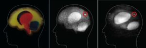
Figure 7. A comparison of the phantom gelatin brain (left), the shielded ultra-low field MRI (center) and the unshielded ultra-low field MRI (right). The red circles indicate simulated regions of bleeding (center, and left). The shielded, ultra-low field MRI image (center) shows enough resolution to identify the major parts of the phantom brain as well as the simulated region of bleeding (circled). The unshielded battlefield MRI (right) has significantly less resolution; however, the bleeding is still visible, indicating that this system might be enough for a doctor in the field to determine the next step in treatment, from Reference 24. (Released)
Discussion and conclusions
A ultra-low field MRI system that is sensitive to anatomical features of interest including regions of bleeding has been developed. While the image quality will likely never compete with traditional MRI, as seen in Figure 5, the ultra-low field MRI system that is a footprint that is conducive to being delivered by a truck or light vehicle and does not require heavy magnets or shielding. This makes for a system is radically different from traditional MRI. Another significant benefit is that the fields can be completely removed for safety. Finally, the low fields (even the 100 mT pre-polarization field) are not adequate to put significant force on metal. Unlike high field MRI, where even a hair pin can be accelerated to 40 mph, it is relatively safe to use in the presence of metal. This means that MRI can be performed in the presence of medical equipment, or on subjects that may contain metal implants or fragments. The low measurement field means that imaging can even be performed through metal, which has been demonstrated for an application in using ultra-low field MRI for the screening of liquids at security checkpoints. [29,30] For example, one can perform MRI through unopened soda cans. It has also been shown that ultra-low field MRI combined with x-ray is an incredibly effective method for telling threat liquids from benign liquids in security screening. [31] It is important to note, in fact, that the development of ultra-low field MRI for anatomical imaging and deployable systems for the detection of threat liquids has been very synergistic.
One notable hurdle that remains is that the SQUID sensor still requires a small amount of cryogens (~ 10 L). It is possible to run with cryo-coolers, which would eliminate the need for refilling within a six month maintenance period. Ultimately, however, sensors that are as sensitive as the SQUID but do not require cryogens will be developed. A promising candidate is the atomic magnetometer, which does not require cryogens and relies on laser-based readout of atomic vapors. We have already begun to demonstrate ultra-low field MRI with such sensors. [32] Ultimately, it may be possible to imagine light and portable MRI systems in an ultra-low field regime. And this, in turn, may bring MRI where it has never been able to go before.
About the Author:
Michelle Espy received her Bachelor of Science in physics from the University of California, Riverside, and her doctorate in experimental
nuclear physics from the University of Minnesota. After completing her doctorate she has pursued the application of nuclear physics techniques to biomedical and applied physics research based on detection of weak electromagnetic fields. She has worked for the past 16 years as part of the SQUID team at Los Alamos National Laboratory. She has more than 55 publications since 1996, four patents and several
awards in the field of MEG and ultra-low field NMR and MRI. She was made a Fellow of the American Physical Society in 2015.
References:
[1] Chapter 21: Facts and Figures (2015, April). Magnetic Resonance: A Peer-Reviewed, Critical Introduction (8th ed., Version 8.9).
[2] Clarke J., Hatridge M., & Mößle M. (2007, August). SQUIDDetected Magnetic Resonance Imaging in Microtesla Fields. Annual Review of Biomedical Engineering, 9, 389–413. doi: 10.1146/annurev.bioeng.9.060906.152010
[3] Ubelacker, S. (2009, April 10). More MRI cash helping rich more than poor, study finds. The Globe and Mail.
[4] Centers for Disease Control. Number of magnetic resonance imaging (MRI) units and computed tomography (CT) scanners: Selected countries, selected years 1990-2009. [PDF file].
[5] Bellamy, R.F. (1992). The medical effects of conventional weapons. World Journal of Surgery, 16(5) 888-892.
[6] Marshall, S., Bell, R., Armonda, R., Savitsky, E., & Ling, G. Chapter 8: Traumatic Brain Injury. In M. Lenhart, E. Savitsky, & B. Eastridge (Eds.), Combat Casualty Care: Lessons Learned from OEF and OIF (pp. 343-392).
[7] A tough homecoming: Veterans of Iraq and Afghanistan are returning home with unprecedented physical and mental wounds. (2012, January 20). The Week.
[8] Lee, B., & Newberg, A. (2005). Neuroimaging in Traumatic Brain Imaging. NeuroRx, 2(2), 372-383. doi: 10.1602/neurorx.2.2.372
[9] Zoroya, G. (2014, January 18). MRI machines for treating soldiers pulled from war zone. USA Today.
[10] Clarke, J., & Braginski, A. (Eds.) (2006, March). The SQUID Handbook: Fundamentals and Technology of SQUIDs and SQUID
Systems, Volume I.
[11] Clarke J., Hatridge M., & Mößle M. (2007, August). SQUIDDetected Magnetic Resonance Imaging in Microtesla Fields. Annual Review of Biomedical Engineering, 9, pp. 389–413. doi: 10.1146/annurev.bioeng.9.060906.152010
[12] McDermott, R., Trabesinger, A. H., Muchk, M., Hahan, E. L., Pines, A., & Clarke, J. (2002). Liquid-state NMR and scalar couplings in microtesla magnetic fields. Science, 295, 2247-2249.
[13] Inglis, B., Buckenmaier, K., Sangiorgio, P., Pedersen, A. F., Nichols, M. A., & Clarke, J. (2013, November 26). MRI of the human brain at 130 microtesla. Proceedings of the National Academy of Sciences of the United States of America. 110(48) pp. 19194-19201. doi: 10.1073/pnas.1319334110
[14] Zotev, V. S., Matlashov, A. N., Volegov, P. L., Savukov, I. M., Epsy, M., Mosher, J. J., … Kraus, R. H. (2008, April). Microtesla MRI of the human brain combined with MEG. Journal of Magnetic Resonance. 194(1) pp. 115-120.
[15] Magnelind, P., Gomez, J., Matlashov, A., Owens, T., Sandin, J. H., Volegov, P., & Espy, M. (2011). Co-registration of interleaved MEG and ULF MRI using a 7 Channel low-Tc SQUID system. IEEE Transactions on Applied Superconductivity. 21(3) pp. 456–460.
[16] Vesanen, P. T., Nieminen, J. O., Zevenhoven, K. C., Dabek, J., Parkkonen, L. T., Zhdanov, A. V., … Ilmoniemi, J. R. (2013, June). Hybrid Ultra-Low-Field MRI and Magnetoencephalography System Based on a Commercial Whole-Head Neuromagnetometer. Magnetic Resonance in Medicine. 69(6) pp. 1795-1804. doi: 10.1002/mrm.24413
[17] Myers, W., Slichter, D., Hatridge, M., Bush, S., Moessle, M., McDermott, R., … Clarke, J. (2006). Calculated signal-to-noise ratio of MRI detected with SQUIDs and Faraday detectors in fields from 10 micro Tesla to 1.5 Tesla. Journal of Magnetic Resonance. 186(2). 182-92.
[18] Callaghan, P. T. (1993). Principles of Nuclear Magnetic Resonance Microscopy. New York, NY: Oxford University Press Inc.
[19] Macovski, A. & Conolly, S. (1993, August). Novel approaches to low-cost MRI. Magnetic Resonance in Medicine. 30(2) 221-230.
[20] Matter, N. I., Scott, G. C., Grafendorfer, T., Macovski, A., & Conolly, S. M. (2006, January). Rapid polarizing field cycling in magnetic resonance imaging. IEEE Transactions on Medical Imaging. 25(1) pp. 84-93.
[21] Espy, M. A., Magnelind, P. E., Matlashov, A. N., Newman, S. G., Sandin, H. J., Schultz, L. J., … Volegov, P. L. (2014, October 30). Progress toward a deployable SQUID-based ultra-low field MRI system for anatomical imaging. IEEE Transactions on Applied Superconductivity. 25(3). doi: 10.1109/TASC.2014.2365473
[22] Zotev, V. S., Volegov, P. L., Matlashov, A. N., Espy, M. A., Mosher, J. C., Kraus, R. H. (2008, June). Parallel MRI at microtesla fields. Journal of Magnetic Resonance. 192(2) pp. 197- 208. doi: 10.1016/j.jmr.2008.02.015
[23] Espy, M., Matlashov, A., Volegov, P. (2013, April). SQUIDdetected ultra-low field MRI. Journal of Magnetic Resonance. 229 pp. 127-141. doi: 10.1016/j.jmr.2013.02.009
[24] Epsy, M. ULF MRI book.
[25] Zotev, V., Volegov, P., Matlashov, A., Savukov, I., Owens, T., & Espy, M. (2009). SQUID-based Microtesla MRI for In Vivo Relaxometry of the Human Brain. IEEE Transactions on Applied Superconductivity. 19(3) pp. 823-826.
[26] Determination of Signal-to-Noise Ratio and Image Uniformity for Single-Channel Non-Volume Coils in Diagnostic MR Imaging. (2008). NEMA Standards Publication MS 6-2008.
[27] Espy, M., Flynn, M., Gomez, J., Hanson, C., Kraus, R., Magnelind, P., … Zotev, V. (2010). Ultra-low-field MRI for the detection of liquid explosives. Superconductor Science & Technology. 23(3).
[28] Roylco Brain Mold.
[29] Espy, M., Flynn, M., Gomez, J., Hanson, C., Kraus, R., Magnelind, P., … Zotev, V. (2010). Ultra-low-field MRI for the detection of liquid explosives. Superconductor Science & Technology. 23(3).
[30] Espy, M., Baguisa, S., Dunkerley, D., Magnelind, P., Matlashov, A., Owens, T., … Volegov, P. (2011). Progress on Detection of Liquid Explosives Using Ultra-Low Field MRI. IEEE Transactions on Applied Superconductivity. 21(3) Part 1, pp. 530-533.
[31] Espy, M., Hunter, J., Schultz, L. (2014, June). What’s in that bottle? Physics Today. 67(6) pp. 62-63.
[32] Savukov, I., & Karaulanov, T. (2013, July 22). Magneticresonance imaging of the human brain with an atomic magnetometer. Applied Physics Letters. 103(4):43703.